The data base VIPAS (Vehicle Induced Pressure And Suction) summarizes the results of extensive fullscale measurements, which have been performed within the DFG research project Ru-345/32-1.
Datenbank VIPAS
Die Datenbank VIPAS (Vehicle Induced Pressure
And Suction) fasst die Ergebnisse zusammen, die im Rahmen des
DFG Forschungsvorhabens Ru-345/32-1 in umfassenden Feldmessungen gewonnen
werden konnten.
![]() Die Abbildungen, Skizzen, Zeichnungen und Fotos auf dieser und
nachfolgend aufrufbaren Internetseiten unterliegen dem Urheberrecht.
Die Abbildungen, Skizzen, Zeichnungen und Fotos auf dieser und
nachfolgend aufrufbaren Internetseiten unterliegen dem Urheberrecht.
![]() The pictures, sketches, drawings and photos on this and subsequent
internet pages are copyright protected.
The pictures, sketches, drawings and photos on this and subsequent
internet pages are copyright protected.
funded by
![]()
Project no. Ru 345/32-1
Research period: 2011 - 2014
Prof. Dr.-Ing. Bodo Ruck & Dr. Petr Lichtneger
Laboratory of Building- and Environmental Aerodynamics
Institute for Hydromechanics
Karlsruhe Institute of Technology (KIT)
Kaiserstr. 12
76131 Karlsruhe, Germany
e-mail: bodo.ruck@t-online.de
Project title
Unsteady pressure and suction forces on flat roadside elements induced
by passing vehicles
Abstract
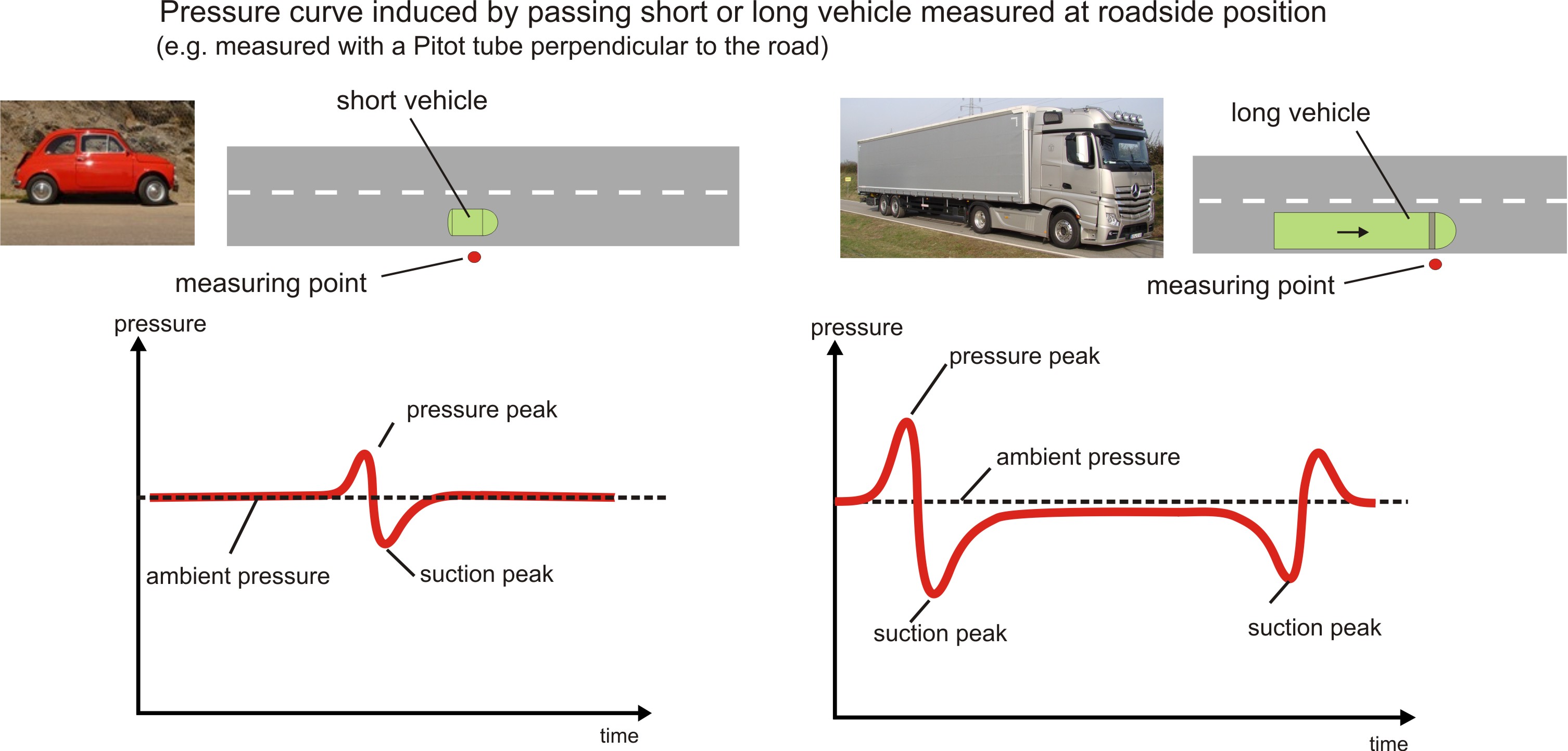
Every day and innumerably, road vehicles of different types pass flat roadside-placed elements like stable or temporary traffic signs, noise barriers, charge devices, etc. The elements are exposed to a vehicle-specific flow and pressure field, i.e. to transient loads. In order to quantify the involved phenomena, full-scale experiments were performed for six different vehicle types and three sizes of square plates, which were aligned in three different configurations with respect to the vehicle's track. For the measurement of loads effecting the plate, the pressure multi-tapping technique was implemented with high temporal and spatial resolution. The experiments delivered a broad data-base for the proper quantification of vehicle induced loads on flat elements as a function of vehicle type, vehicle velocity and passing distance to the plate, element size as well as spatial plate alignment with respect to the vehicle.
Timo Bauer, Dieter Groß, Armin Reinsch, Harald Deutsch
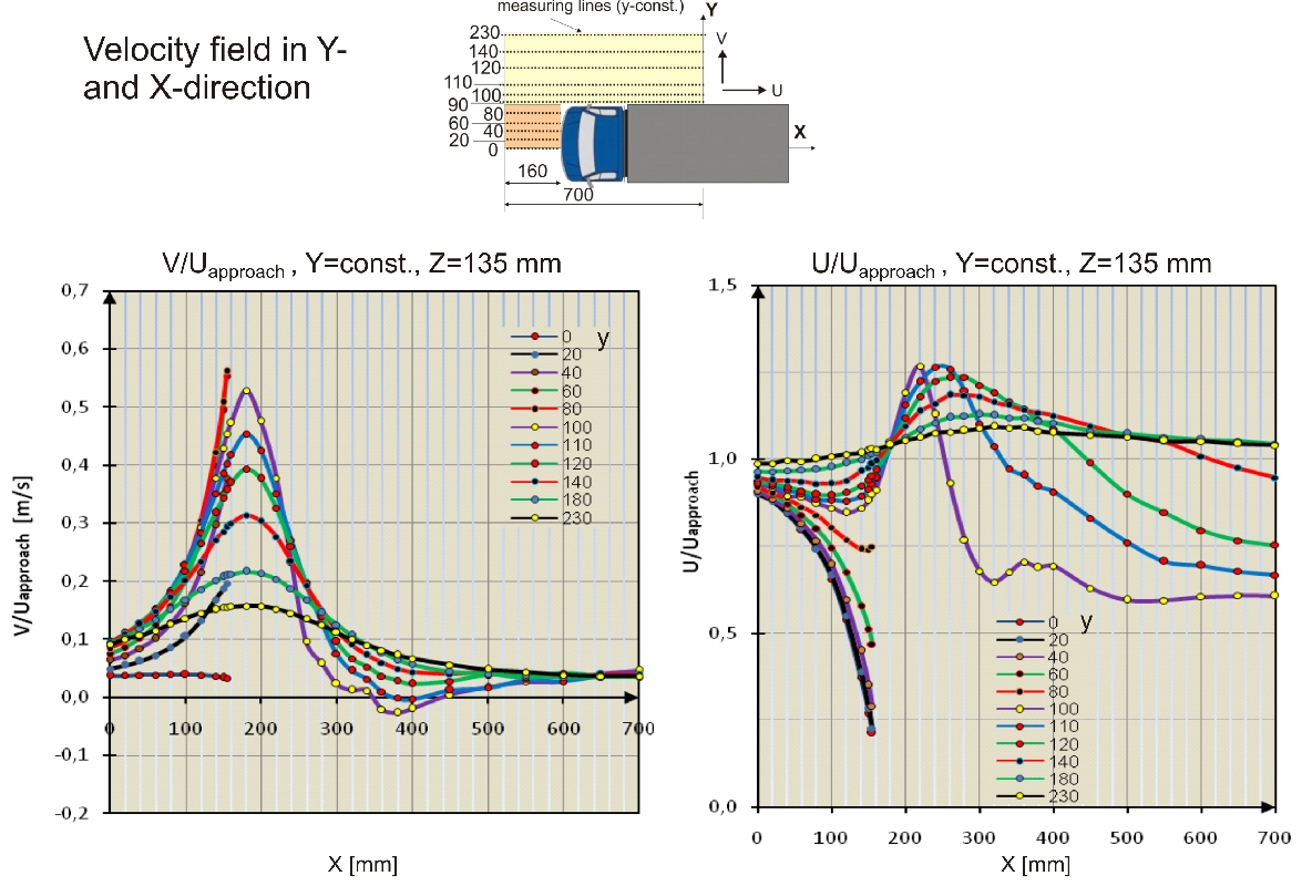
LDA measurements
Dr.-Ing. Boris Pavlovski
Subject of research within project DFG Ru 345/32-1
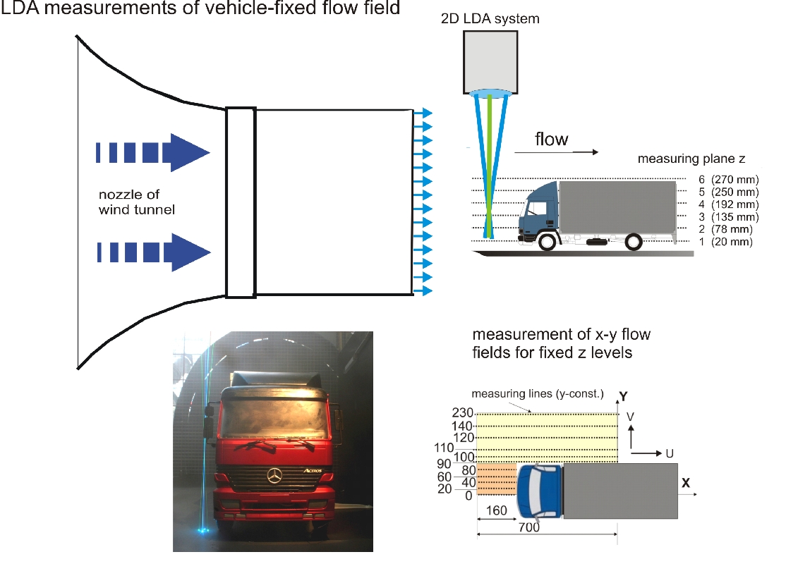
Flow field around a moving vehicle with no interacting roadside element (fundamentals)
How
to imagine the flow field around a box-shaped vehicle ?
(wind tunnel measurements with laser Doppler anemometry)
© B. Ruck
Fullscale investigation: Flow
field around a moving vehicle with interacting roadside element
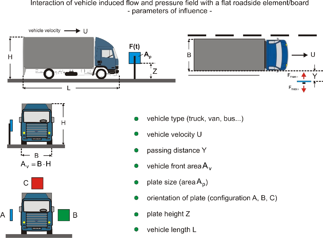
Parameters of influence
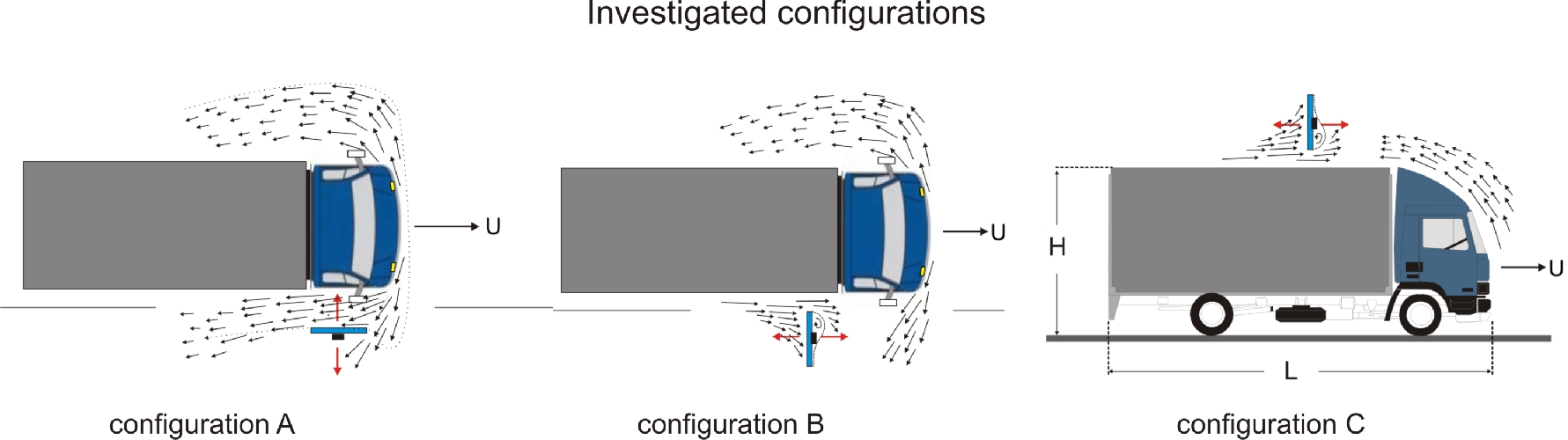
Investigated vehicle types
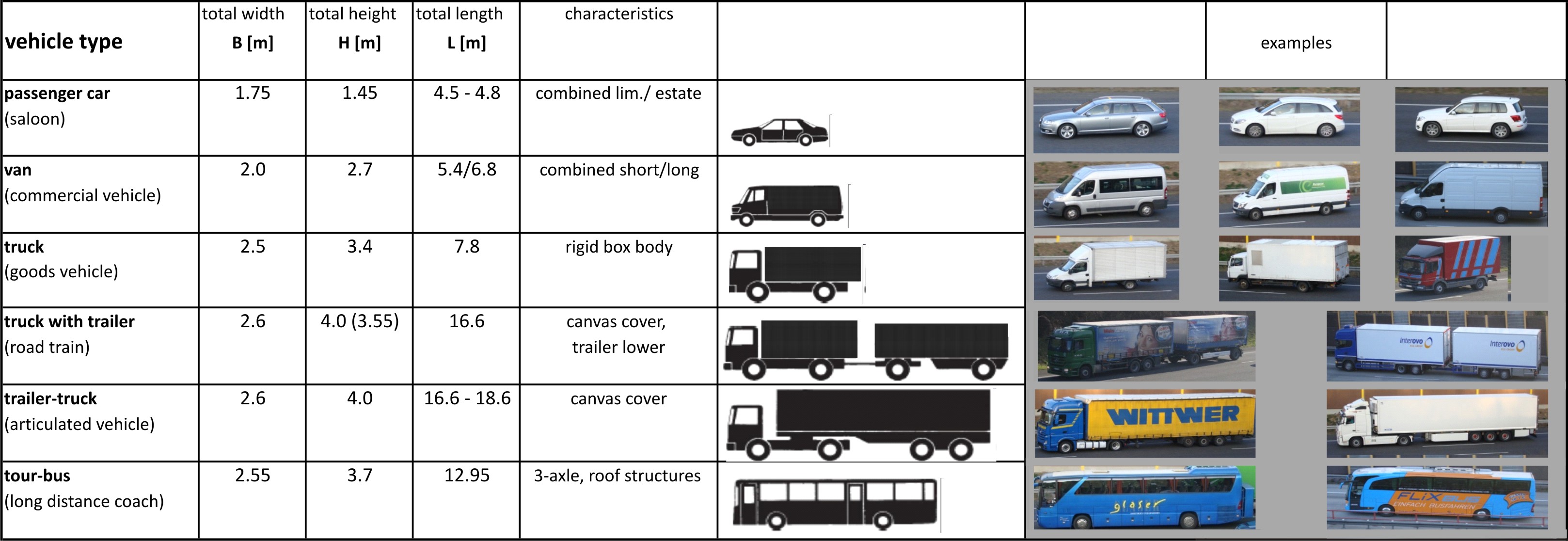
Table 1: Data of vehicle types
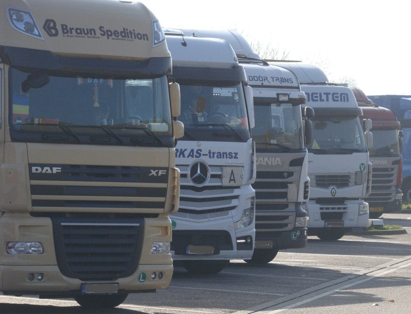
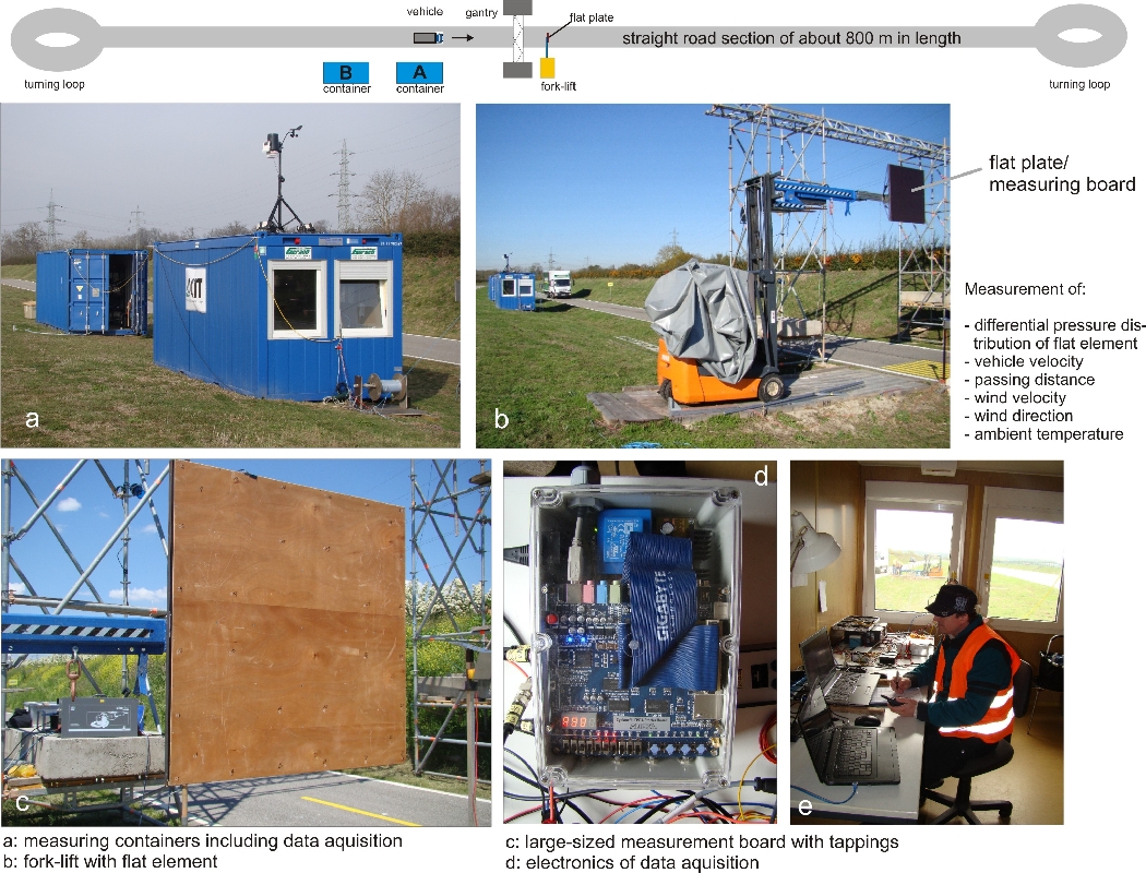
Fullscale measuring campaign - different vehicle types
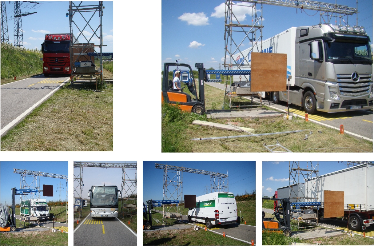
Definitions, dimensions, conventions
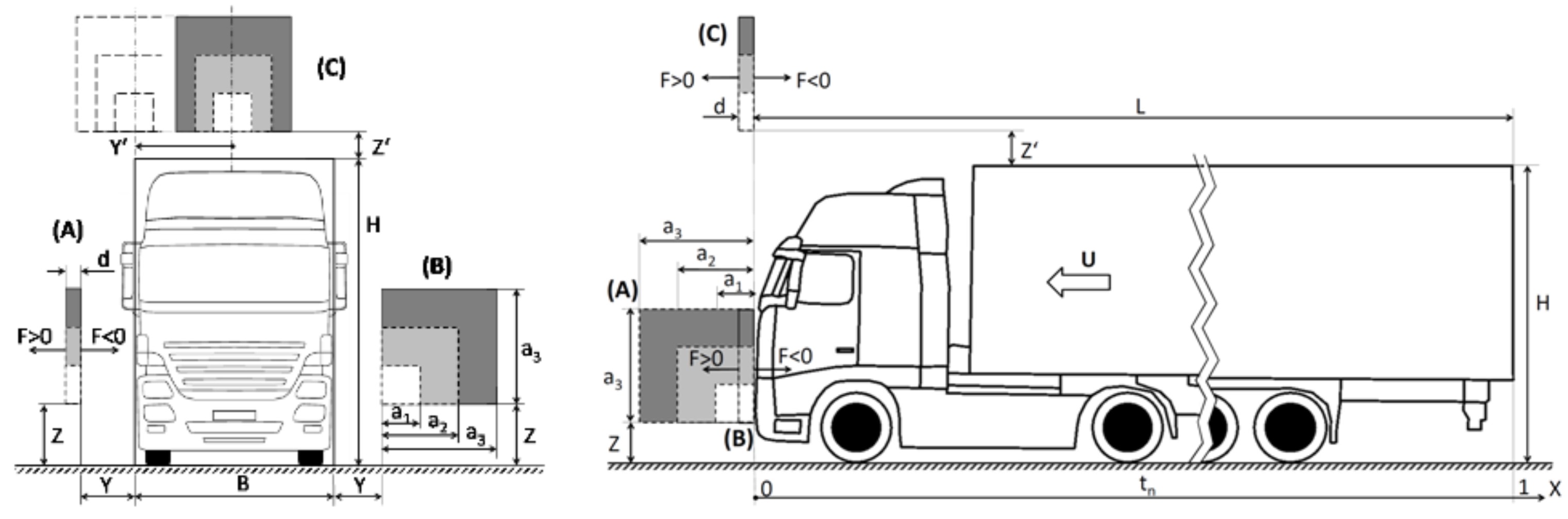
Layout of experiment showing three configurations A, B and C – front
and side
view;
investigated flat element sizes 50 cm x 50 cm, 100 cm x 100 cm or 150 cm x
150 cm, i.e. a1=50 cm, a2=100 cm, a3=150 cm
Data capturing and processing
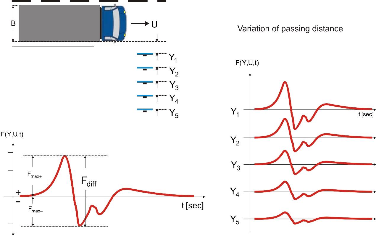
The test plates were equipped with many pressure tappings on both sides in order to measure differential pressure distributions with high spatial and temporal resolution during the vehicle's passing. Integrating the instantaneous differential pressure distribution (pressure difference between front and back side of the flat element) leads to a transient force acting on the element, which is a function of vehicle type, passing distance Y, vehicle velocity U and time t. These time-dependent force curves are given examplarily in the following figure for all three configurations (A, B, C):
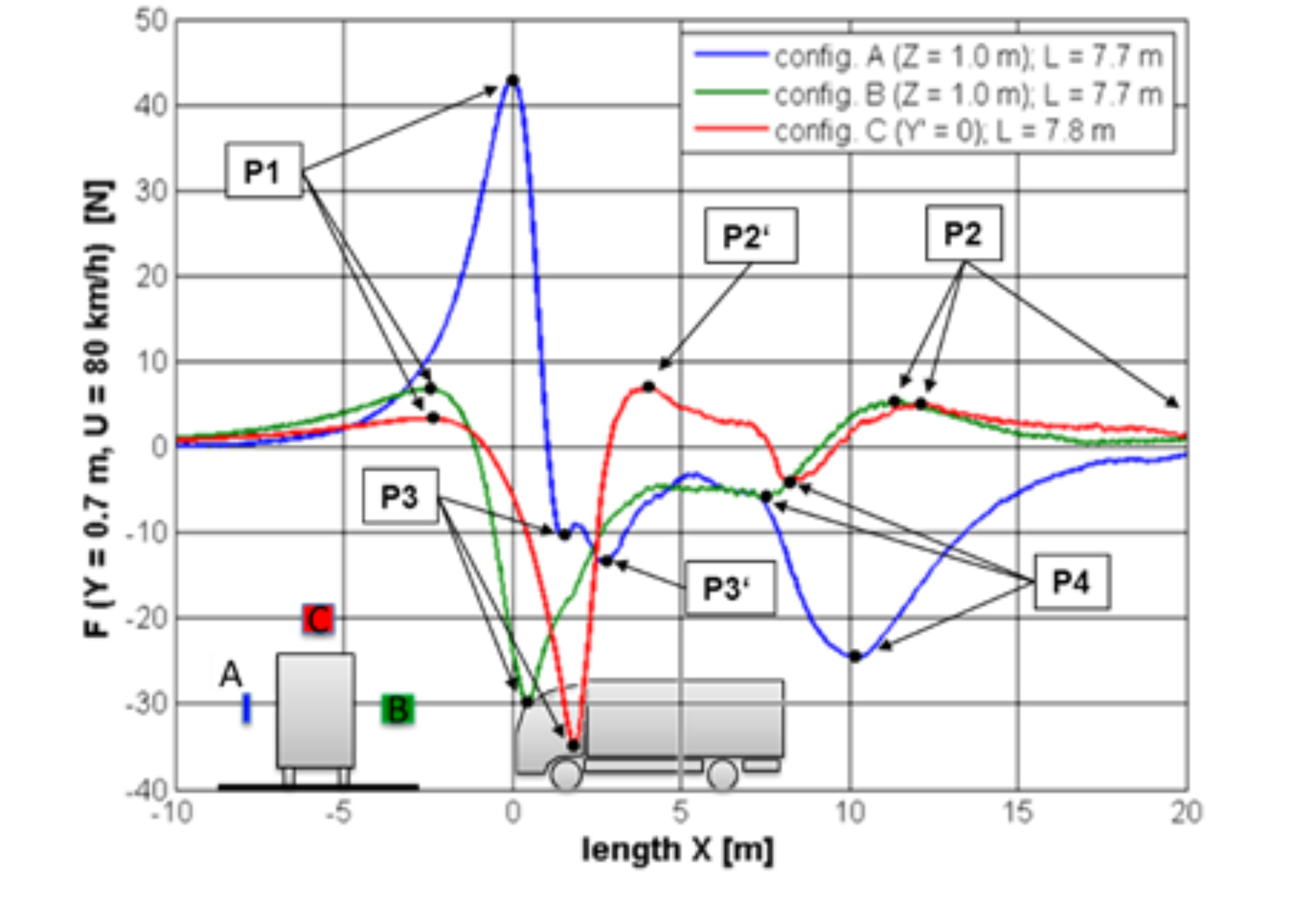
Fig. 1:
Characteristic force curves measured with truck and different configurations
A, B, C; medium-sized plate; ensemble averaged curves, re-calculated for a
passing distance of 0.7 m and an approach velocity of 80 km/h using the
appropriate distance model as described below.
Please note:
A
'test
position'
is
defined as a combination of one particular configuration
(A, B, or C),
one
vehicle type,
one
vertical level Z of the test plate.
Ui and Yi vary during the fullscale experiments
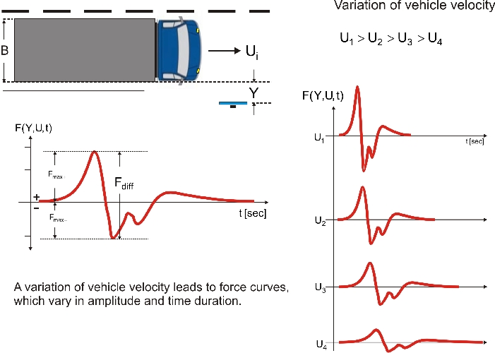
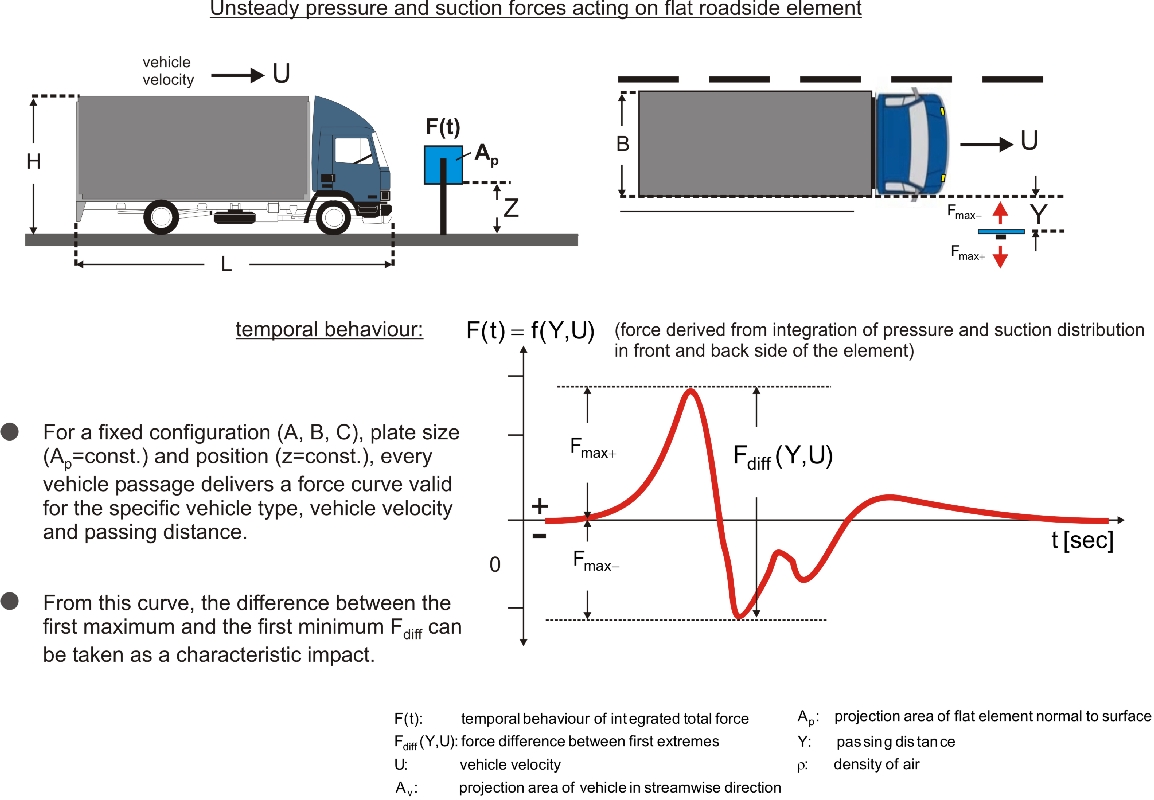
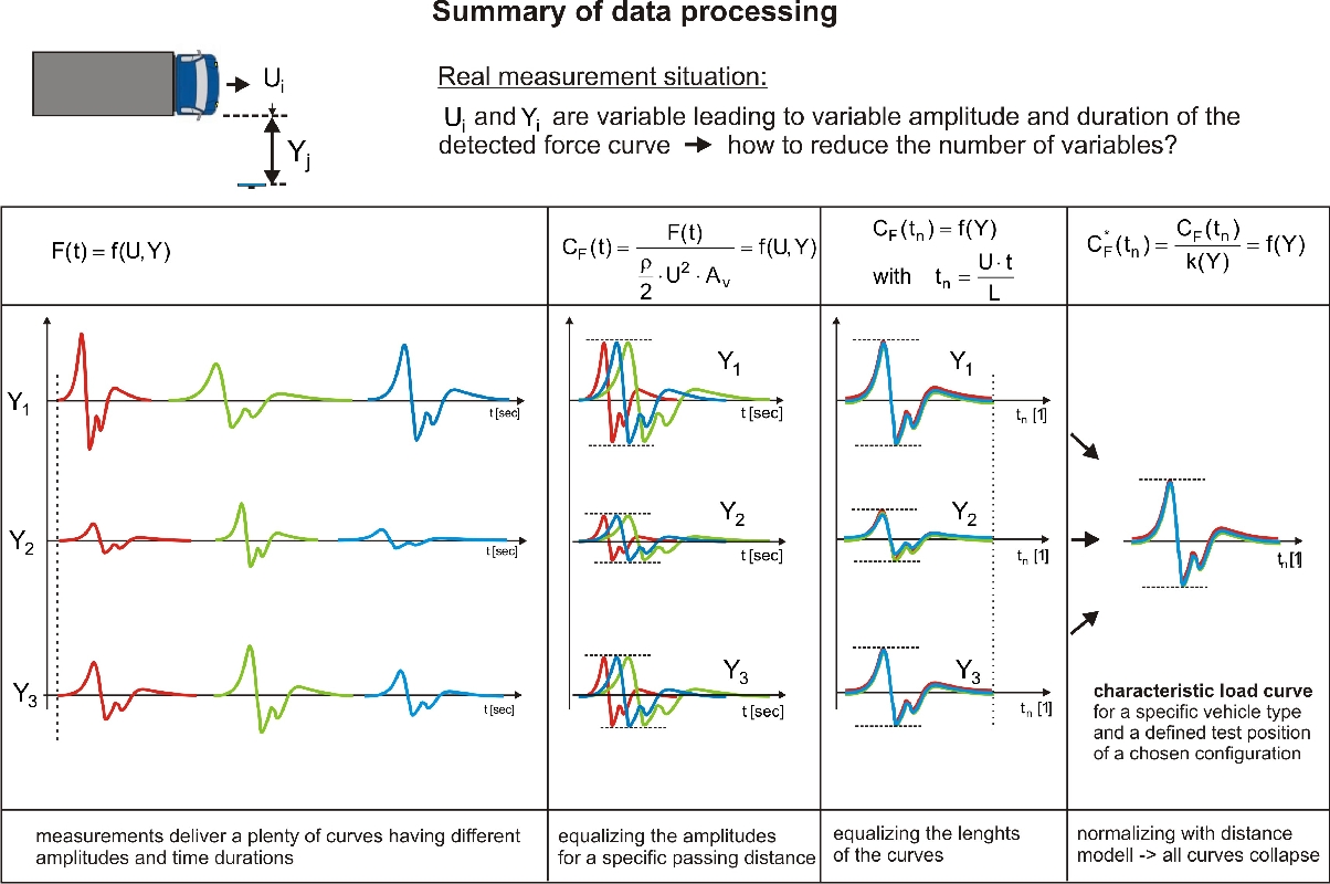
Since wind loads depend on the square of velocity, the vehicle-induced force F(t) was normalized by a force consisting of the product of vehicle velocity-based dynamic pressure, air density and the vehicle frontal area (Av = B x H). This led to the dimensionless transient force coefficient CF(t).
The curves for the dimensionless transient force coefficient CF (t) still depend on U and Y, however, all curves of the same passing distance show the same amplitude but have different time durations due to varying vehicle velocity. If we introduce on the abscissa a dimensionless time tn formed by multiplying the real time with the vehicle velocity divided by the vehicle length L, then, all measured curves of the dimensionless transient force coefficient CF(tn) will have the same length. Thus, for a fixed passing distance Y, the curves of CF(tn) show the same amplitude, i.e. CF(tn) depends only on Y
Since the dimensionless transient force coefficient CF(tn) depends only on Y, it should be possible to divide it by a function k(Y), which is called 'distance model', forcing all curves collapsing to more or less one single curve, the 'characteristic load curve' for one test position, see below..
The distance model describes the relation between force impact and passing distance Y. In order to obtain a distance model, a great number of vehicle passings was realized with a specified test position measuring the differential force coefficient (difference of the force coefficient of the first maximum P1 and first minimum P3, see Fig. 1) in each curve and display the values in a graph. It was found that the differential force coefficient CF,diff13 could be approximated with a 3rd power function fitted within the tested distance range. Thus, for each test position, a distance model k(Y) was estimated applying model coefficients a [m3] and b [m] appropriately.
![]()
The decay with power of -3 corresponds to a simplified theoretical model presented in Sanz-Andrés et al. 1992 (Sanz-Andrés, A., Laverón, A., Quinn, A., Vehicle induced loads on pedestrian barriers’, Journal of Wind Eng. & Ind. Aerodyn., 2003, 92, pp. 413-442). In the following Figure 2, values of differential force coefficients CF,diff13 based on force measurements with a truck are displayed. As can be seen, three distance models k(Y) for the three different configurations (A, B, C) can be derived by fitting a curve to the measurement points. The distance models (curves) increasingly differ with decreasing passing distance. For greater distances, the curves tend to zero, which means that the impact on the plate due to a passing vehicle is vanishing.
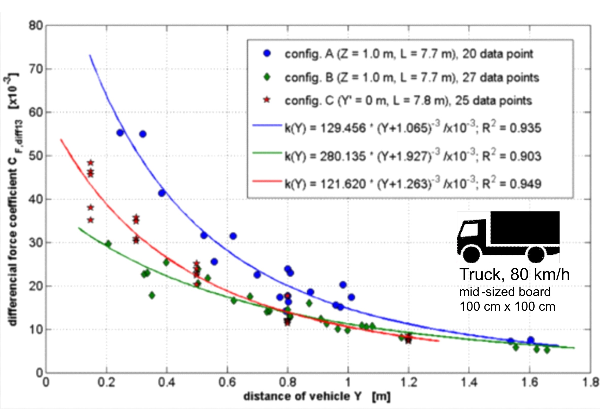
Fig. 2:
Differential force coefficient
(characterizing the force jump between the first maximum and first minimum
of a detected force curve) depending
on passing distance of vehicle with respect to testing plate. Fitting of
curves (distance models) to the measurement values
for three truck test positions (for configuration C the notation of distance
Y symbolizes vertical distance Z’); R² coefficient of determination.
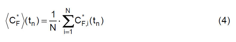
As explained before, the curves of the dimensionless force coefficient CF(tn) were normalized with the distance models k(Y). Additionally, all runs of a single test position were ensemble averaged (please note again that a 'test position' is defined as a combination of one particular configuration (A, B, or C), one vehicle type, one vertical level Z of the test plate).
In this way, the aforementioned characteristic load curves could be obtained for each test position, see VIPAS data below. Because the distance model was set up using the bow wave loading peaks (peak P1 and P3), a single force curve behind these peaks can more or less deviate from the characteristic load curve in dependence on the current distance.
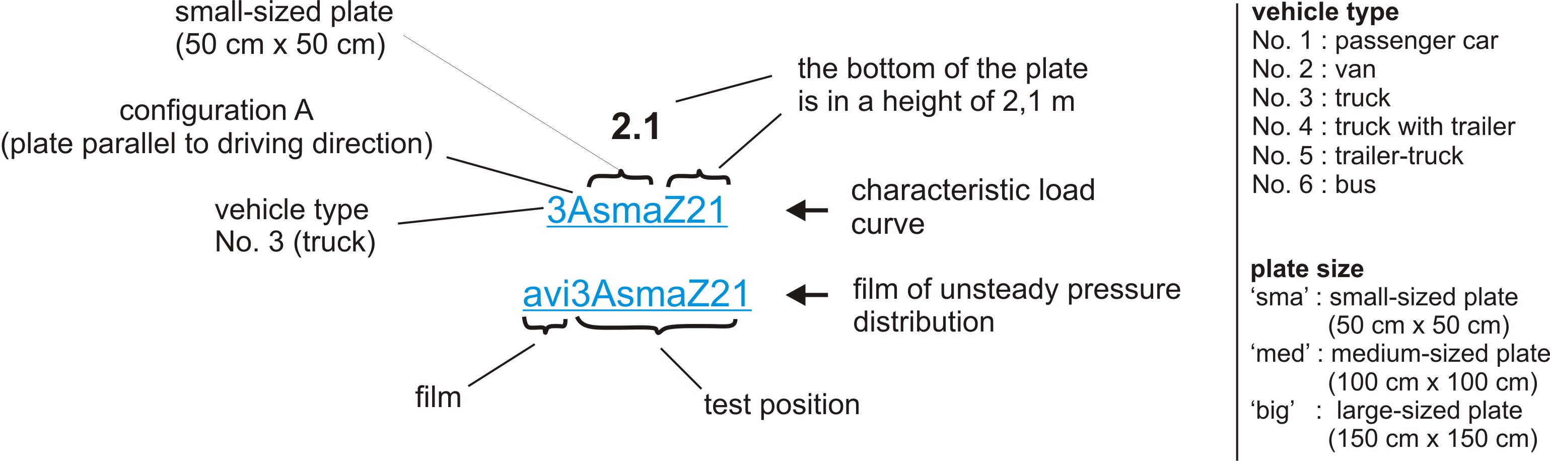
VIPAS data - part 1: flat plate
A 'test position' is defined as a combination of one particular configuration (A, B, or C), one vehicle type and one vertical level Z of the test plate. At each test position, typically, N = 15 to 25 test runs were carried out. For each run, the variable vehicle velocity U and the variable distance Y between plate and vehicle were captured automatically using laser light beam trigger and distance measuring technique.
In the following tables 2-4, the main results of the fullscale experiments are given. Each box of the tables (except the last column) denotes a test position and contains two files. The upper one shows the characteristic load curve of the test position and the lower one shows the unsteady differential pressure distribution (difference between front- and backpressure) at the flat plate induced by the passing vehicle. The last column gives a comparison of the induced force acting on the element for different vehicle types but with the same testing plate configuration, the same testing plate size and the same testing plate height.
Example 1:
Let an examplary test position be defined by the combination of "truck", "configuration
A", "plate size Ap" (50 cm x 50 cm) and "plate height Z" (=2,1
m). Then, this leads to a box in
table 2 containing the information:
|
A = (50x50) cm2 |
vehicle type |
comparison |
||||||
|
configuration |
variable |
No. 1 |
No. 2 |
No. 3 |
No. 4 |
No. 5 |
No. 6 |
comp. code |
|
(A) |
Z [m] (position code) |
|||||||
|
0.5 |
0.5-0.7 |
0.7 |
- |
- |
- |
|||
|
1.0 |
1.0 |
1.4 |
1.4 |
1.8 |
1.5 |
|||
|
1.5 |
1.4-1.5 |
|||||||
|
- |
2.1 |
2.1 |
- |
- |
||||
|
- |
2.8 |
2.8 |
3.4 |
3.4 |
3.2 |
|||
|
(B) |
Z [m] (position code) |
|||||||
|
0.5 |
0.5-0.7 |
0.7 |
- |
- |
- |
|||
|
1.0 |
1.0 |
1.5-1.7 |
1.8 |
1.8 |
1.5 |
|||
|
1.5 |
1.5-1.7 |
|||||||
|
- |
2.1 |
2.1 |
- |
|||||
|
- |
2.8 |
2.8 |
3.4 |
3.4 |
3.2 |
|||
|
(C) |
Y’ [m] (position code) |
|||||||
|
» B/2 |
» B/2 |
» B/2 |
- |
- |
- |
|||
|
Note: In the given distance models for configuration C, Y=Z' Ranges of variables accomplished within measurements |
|
|||||||
|
(A) (B) (C) |
U [km/h] |
» 40-100 |
» 40-100 |
» 40-90 |
» 50-80 |
» 50-80 |
» 50-80 |
|
|
(A) (B) |
Y [m] |
» 0.3 - 1.9 |
» 0.2 - 1.6 |
» 0.3 - 1.5 |
» 0.4 - 2 |
» 0.4 - 2 |
» 0.3 - 2 |
|
|
(C) |
Z’ [m] |
» 0.2 - 1.1 |
» 0.15-1.1 |
» 0.15-1.2 |
» 0.1 - 1.3 |
» 0.1 - 1.3 |
» 0.15-0.8 |
|
Table 2: Results of measurement series with
the small-sized testing board
back
|
Ap = (100x100) cm2 |
vehicle type |
comparison |
||||||
|
configuration |
variable |
No. 1 |
No. 2 |
No. 3 |
No. 4 |
No. 5 |
No. 6 |
comp. code |
|
(A) |
Z [m] (position code) |
|||||||
|
0.7 |
1.0 |
1.0 |
1.5 |
1.5 |
1.0 |
|||
|
1.4 |
2.0 |
2.0 |
||||||
|
- |
3.0 |
3.0 |
3.1 |
3.0 |
2.9 |
|||
|
(B) |
Z [m] (position code) |
|||||||
|
0.7 |
1.0 |
1.0 |
1.5 |
1.5 |
1.0 |
|||
|
1.4 |
2.0 |
2.0 |
||||||
|
- |
3.0 |
3.0 |
3.0 |
3.0 |
2.9 |
|||
|
(C) |
Y’ [m] (position code) |
|||||||
|
»
B/2 |
»
B/2 |
»
B/2 |
- |
- |
- |
|||
|
Note: In the given distance models for configuration C, Y=Z' Ranges of variables accomplished within measurements |
|
|||||||
|
(A) (B) (C) |
U [km/h] |
» 50-100 |
» 50-100 |
» 40-90 |
» 40-80 |
» 40-80 |
» 50-90 |
|
|
(A) (B) |
Y [m] |
» 0.3 - 2 |
» 0.3 - 1.6 |
» 0.2 - 1.6 |
» 0.4 - 2 |
» 0.4 - 2 |
» 0.3 - 2 |
|
|
(C) |
Z’ [m] |
» 0.2-1.05 |
» 0.15-1.1 |
» 0.15-1.2 |
» 0.1 - 1.1 |
» 0.1 - 1.1 |
» 0.15 - 1 |
|
Table 3: Results of measurement series with
the medium-sized testing board
back
|
Ap = (150x150) cm2 |
vehicle type |
comparison |
||||||
|
configuration |
variable |
No. 1 |
No. 2 |
No. 3 |
No. 4 |
No. 5 |
No. 6 |
comp. code |
|
(A) |
Z [m] (position code) |
|||||||
|
1.0 |
1.0 |
1.0 |
1.0 |
1.0 |
1.0 |
|||
|
- |
- |
2.8 |
2.5 |
2.5 |
2.5 |
|||
|
(B) |
Z [m] (position code) |
|||||||
|
1.0 |
1.0 |
1.0 |
1.0 |
1.0 |
1.0 |
|||
|
- |
- |
2.5 |
2.5 |
2.5 |
2.5 |
|||
|
(C) |
Y’ [m] (position code) |
|||||||
|
Note: In the given distance models for configuration C, Y=Z' Ranges of variables accomplished within measurements |
|
|||||||
|
(A) (B) (C) |
U [km/h] |
» 50-100 |
» 50-100 |
» 40-90 |
» 40-80 |
» 40-80 |
» 40-80 |
|
|
(A) (B) |
Y [m] |
» 0.3 - 2.5 |
» 0.3 - 2.5 |
» 0.4 - 2.1 |
» 0.4 - 2 |
» 0.4 - 2 |
» 0.3 - 2 |
|
|
(C) |
Z’ [m] |
» 0.1 - 1 |
» 0.2-1.15 |
» 0.1 - 0.9 |
» 0.15-1.1 |
» 0.15-1.1 |
» 0.15-0.6 |
|
Table 4: Results of measurement series with
the large-sized testing board
How to use data base VIPAS - part 1: flat plate
Supposed, the passing distance Y, the vehicle velocity U and the vehicle type with frontal area Av are known, the data base VIPAS can be used to compute the wind load F(t) or F(X) acting on a flat element of size 50 cm x 50 cm, 100 cm x 100 cm or 150 cm x 150 cm in height Z with configuration A, B or C. This computation can be performed on the basis of the experimentally determined characteristic load curves <CF*> in combination with the distance models k(Y) derived from full scale measurements:
Substituting tn with Eq. (2) delivers the resultant force F(t) or F(X).
Example 2: Which is the maximum force acting
on a plate element of size 100 cm x 100 cm (medium-sized plate) with
configuration A and a plate height of Z=3,0 m induced by a trailer-truck
(No. 5) with velocity U=90 km/h and a passing distance of Y=0,4 m ?
Thus, the corresponding file code is "5AmedZ30", which can be found in Table
3 and delivers the following characteristic load curve:
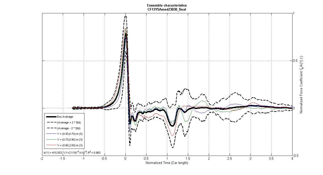
From this characteristic load curve (black), one can infer that the maximum normalized force coefficient reaches a positive value of about 0.75 and the corresponding distance model is given in the lower left corner. The frontal area of the trailer-truck can be inferred from Table 1. Thus, for this particular test position the computation is as follows:
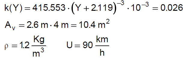
Inserting these values into equation (5) delivers
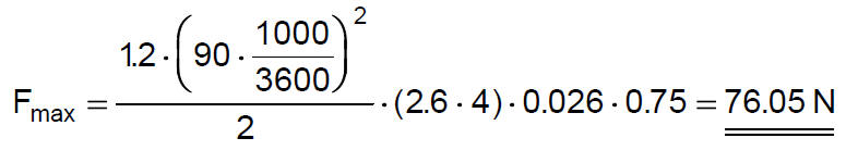
As a result, a maximum pressure force (away from the vehicle) of about 76 N is acting on the testing plate of size 100 cm x 100 cm.
![]() Data and images contained within this database are subject to copyright and
are published for non-commercial use only. The user is not entitled to use
the data commercially or publish the database or any part therof.
Data and images contained within this database are subject to copyright and
are published for non-commercial use only. The user is not entitled to use
the data commercially or publish the database or any part therof.
![]() Die Daten und Inhalte der Datenbasis VIPAS sind urheberrechtlich geschützt.
Die Veröffentlichung in Form dieser Website dient ausschließlich der
persönlichen Information. Eine kommerzielle Verwendung/Verwertung der in der
Datenbasis enthaltenen Informationen ist nicht zulässig. Ebenso nicht
zulässig ist eine Veröffentlichung oder Vervielfältigung der auf dieser
Website gespeicherten Informationen durch Besucher/Nutzer.
Die Daten und Inhalte der Datenbasis VIPAS sind urheberrechtlich geschützt.
Die Veröffentlichung in Form dieser Website dient ausschließlich der
persönlichen Information. Eine kommerzielle Verwendung/Verwertung der in der
Datenbasis enthaltenen Informationen ist nicht zulässig. Ebenso nicht
zulässig ist eine Veröffentlichung oder Vervielfältigung der auf dieser
Website gespeicherten Informationen durch Besucher/Nutzer.
Disclaimer/Haftungsausschluss
![]() The data, text, graphics and links contained in these pages are provided for
information purposes only. The authors provide no warranty, expressed or
implied, as to the accuracy, reliability, or completeness of the data, text,
links, and other items contained on these pages and exclude any
responsibility for loss which may arise from reliance on data contained in
this database. The authors may make changes to the data contained in these
pages at any time without notice. The authors reserve the right to modify or
withdraw, temporarily or permanently, the database (or any part thereof)
without notice.
The data, text, graphics and links contained in these pages are provided for
information purposes only. The authors provide no warranty, expressed or
implied, as to the accuracy, reliability, or completeness of the data, text,
links, and other items contained on these pages and exclude any
responsibility for loss which may arise from reliance on data contained in
this database. The authors may make changes to the data contained in these
pages at any time without notice. The authors reserve the right to modify or
withdraw, temporarily or permanently, the database (or any part thereof)
without notice.
![]() Die Inhalte dieser Datenbasis wurden mit größtmöglicher Sorgfalt erstellt.
Die Autoren übernehmen jedoch keine Gewähr für die Richtigkeit und
Vollständigkeit der bereitgestellten Inhalte. Die Nutzung der Inhalte der
Datenbasis erfolgt auf eigene Gefahr des Nutzers. Ebenso wird keinerlei
Haftung übernommen für jeglichen mittelbaren oder unmittelbaren Schaden
welcher Art auch immer, der sich aus der Nutzung der Datenbank ergeben
sollte. Die Autoren behalten sich vor, die Datenbank jederzeit und ohne
Vorankündigung zu modifizieren oder teilweise oder gänzlich zurückzuziehen
und abzuschalten.
Die Inhalte dieser Datenbasis wurden mit größtmöglicher Sorgfalt erstellt.
Die Autoren übernehmen jedoch keine Gewähr für die Richtigkeit und
Vollständigkeit der bereitgestellten Inhalte. Die Nutzung der Inhalte der
Datenbasis erfolgt auf eigene Gefahr des Nutzers. Ebenso wird keinerlei
Haftung übernommen für jeglichen mittelbaren oder unmittelbaren Schaden
welcher Art auch immer, der sich aus der Nutzung der Datenbank ergeben
sollte. Die Autoren behalten sich vor, die Datenbank jederzeit und ohne
Vorankündigung zu modifizieren oder teilweise oder gänzlich zurückzuziehen
und abzuschalten.
Publications
Lichtneger, P., Ruck, B., 2013: "Transient wind loads on flat elements induced by passing vehicles", Proc. 21. Fachtagung „Lasermethoden in der Strömungsmesstechnik”, Universität der Bundeswehr München, ISBN 978-3-9805613-9-6, ISSN 2194-2447
Lichtneger, P., Ruck, B., 2015: "Full scale experiments on vehicle induced transient loads on roadside plates", Journal of Wind Engineering & Industrial Aerodynamics, 136, 73-81
Lichtneger, P., Ruck, B., 2014: "Transient wind loads on roadside-mounted and overhanging flat elements induced by passing vehicles", First international conference in numerical and experimental aerodynamics of road vehicles and trains (Aerovehicles 1), Bordeaux, France, June 23-25, 2014